CUSTOMER RESPONSE PREDICTION
> str(iris)'data.frame': 150 obs. of 5 variables:
$ Sepal.Length: num 5.1 4.9 4.7 4.6 5 5.4 4.6 5 4.4 4.9 ...
$ Sepal.Width : num 3.5 3 3.2 3.1 3.6 3.9 3.4 3.4 2.9 3.1 ...
$ Petal.Length: num 1.4 1.4 1.3 1.5 1.4 1.7 1.4 1.5 1.4 1.5 ...
$ Petal.Width : num 0.2 0.2 0.2 0.2 0.2 0.4 0.3 0.2 0.2 0.1 ...
$ Species : Factor w/ 3 levels "setosa","versicolor",..: 1 1 1 1 1 1 1 1 1 1 ...
> attributes(iris)
$`names`
[1] "Sepal.Length" "Sepal.Width" "Petal.Length"
[4] "Petal.Width" "Species"
$class
[1] "data.frame"
$row.names
[1] 1 2 3 4 5 6 7 8 9 10 11 12 13 14
[15] 15 16 17 18 19 20 21 22 23 24 25 26 27 28
[29] 29 30 31 32 33 34 35 36 37 38 39 40 41 42
[43] 43 44 45 46 47 48 49 50 51 52 53 54 55 56
[57] 57 58 59 60 61 62 63 64 65 66 67 68 69 70
[71] 71 72 73 74 75 76 77 78 79 80 81 82 83 84
[85] 85 86 87 88 89 90 91 92 93 94 95 96 97 98
[99] 99 100 101 102 103 104 105 106 107 108 109 110 111 112
[113] 113 114 115 116 117 118 119 120 121 122 123 124 125 126
[127] 127 128 129 130 131 132 133 134 135 136 137 138 139 140
[141] 141 142 143 144 145 146 147 148 149 150
> iris[1:5,]
Sepal.Length Sepal.Width Petal.Length Petal.Width Species
1 5.1 3.5 1.4 0.2 setosa
2 4.9 3.0 1.4 0.2 setosa
3 4.7 3.2 1.3 0.2 setosa
4 4.6 3.1 1.5 0.2 setosa
5 5.0 3.6 1.4 0.2 setosa
>
> head(iris)
Sepal.Length Sepal.Width Petal.Length Petal.Width Species
1 5.1 3.5 1.4 0.2 setosa
2 4.9 3.0 1.4 0.2 setosa
3 4.7 3.2 1.3 0.2 setosa
4 4.6 3.1 1.5 0.2 setosa
5 5.0 3.6 1.4 0.2 setosa
6 5.4 3.9 1.7 0.4 setosa
> tail(iris)
Sepal.Length Sepal.Width Petal.Length Petal.Width
145 6.7 3.3 5.7 2.5
146 6.7 3.0 5.2 2.3
147 6.3 2.5 5.0 1.9
148 6.5 3.0 5.2 2.0
149 6.2 3.4 5.4 2.3
150 5.9 3.0 5.1 1.8
Species
145 virginica
146 virginica
147 virginica
148 virginica
149 virginica
150 virginica
> iris[1:10, "Sepal.Length"]
[1] 5.1 4.9 4.7 4.6 5.0 5.4 4.6 5.0 4.4 4.9
> iris$Sepal.Length[1:10]
[1] 5.1 4.9 4.7 4.6 5.0 5.4 4.6 5.0 4.4 4.9
> summary(iris)
Sepal.Length Sepal.Width Petal.Length
Min. :4.300 Min. :2.000 Min. :1.000
1st Qu.:5.100 1st Qu.:2.800 1st Qu.:1.600
Median :5.800 Median :3.000 Median :4.350
Mean :5.843 Mean :3.057 Mean :3.758
3rd Qu.:6.400 3rd Qu.:3.300 3rd Qu.:5.100
Max. :7.900 Max. :4.400 Max. :6.900
Petal.Width Species
Min. :0.100 setosa :50
1st Qu.:0.300 versicolor:50
Median :1.300 virginica :50
Mean :1.199
3rd Qu.:1.800
Max. :2.500
> quantile(iris$Sepal.Length)
0% 25% 50% 75% 100%
4.3 5.1 5.8 6.4 7.9
> quantile(iris$Sepal.Length, c(.1, .3, .65))
10% 30% 65%
4.80 5.27 6.20
> var(iris$Sepal.Length)
[1] 0.6856935
> var(iris$Sepal.Length)
[1] 0.6856935
> hist(iris$Sepal.Length)
> plot(density(iris$Sepal.Length))
> table(iris$Species)
setosa versicolor virginica
50 50 50
> pie(table(iris$Species))
> barplot(table(iris$Species))
>
> cov(iris$Sepal.Length, iris$Petal.Length)
[1] 1.274315
>
> cov(iris[,1:4])
Sepal.Length Sepal.Width Petal.Length
Sepal.Length 0.6856935 -0.0424340 1.2743154
Sepal.Width -0.0424340 0.1899794 -0.3296564
Petal.Length 1.2743154 -0.3296564 3.1162779
Petal.Width 0.5162707 -0.1216394 1.2956094
Petal.Width
Sepal.Length 0.5162707
Sepal.Width -0.1216394
Petal.Length 1.2956094
Petal.Width 0.5810063
>
> cor(iris$Sepal.Length, iris$Petal.Length)
[1] 0.8717538
>
> cor(iris[,1:4])
Sepal.Length Sepal.Width Petal.Length
Sepal.Length 1.0000000 -0.1175698 0.8717538
Sepal.Width -0.1175698 1.0000000 -0.4284401
Petal.Length 0.8717538 -0.4284401 1.0000000
Petal.Width 0.8179411 -0.3661259 0.9628654
Petal.Width
Sepal.Length 0.8179411
Sepal.Width -0.3661259
Petal.Length 0.9628654
Petal.Width 1.0000000
> aggregate(Sepal.Length ~ Species, summary, data=iris)
Species Sepal.Length.Min. Sepal.Length.1st Qu.
1 setosa 4.300 4.800
2 versicolor 4.900 5.600
3 virginica 4.900 6.225
Sepal.Length.Median Sepal.Length.Mean Sepal.Length.3rd Qu.
1 5.000 5.006 5.200
2 5.900 5.936 6.300
3 6.500 6.588 6.900
Sepal.Length.Max.
1 5.800
2 7.000
3 7.900
> boxplot(Sepal.Length~Species, data=iris)
> with(iris, plot(Sepal.Length, Sepal.Width, col=Species, pch=as.numeric(Species)))
>
> plot(jitter(iris$Sepal.Length), jitter(iris$Sepal.Width))
> pairs(iris)
> library(scatterplot3d)
> scatterplot3d(iris$Petal.Width, iris$Sepal.Length, iris$Sepal.Width)
> library(rgl)
Warning message:
package ‘rgl’ was built under R version 3.5.1
> detach("package:rgl", unload=TRUE)
> library("rgl", lib.loc="~/R/win-library/3.5")
Warning message:
package ‘rgl’ was built under R version 3.5.1
> library(rgl)
> plot3d(iris$Petal.Width, iris$Sepal.Length, iris$Sepal.Width)
> distMatrix <- as.matrix(dist(iris[,1:4]))
> heatmap(distMatrix)
>
> library(lattice)
> levelplot(Petal.Width~Sepal.Length*Sepal.Width, iris, cuts=9,
+ col.regions=grey.colors(10)[10:1])
> filled.contour(volcano, color=terrain.colors, asp=1,
+ plot.axes=contour(volcano, add=T))
>
> persp(volcano, theta=25, phi=30, expand=0.5, col="lightblue")
> library(MASS)
>
> parcoord(iris[1:4], col=iris$Species)
>
>
> library(lattice)
> parallelplot(~iris[1:4] | Species, data=iris)
>
> library(ggplot2)
Warning message:
package ‘ggplot2’ was built under R version 3.5.1
> qplot(Sepal.Length, Sepal.Width, data=iris, facets=Species ~.)
>
> myFormula <- Species ~ Sepal.Length + Sepal.Width + Petal.Length + Petal.Width
object 'trainData' not found
> set.seed(1234)
> ind <- sample(2, nrow(iris), replace=TRUE, prob=c(0.7, 0.3))
> trainData <- iris[ind==1,]
> testData <- iris[ind==2,]
> iris_ctree <- ctree(myFormula, data=trainData)
> table(predict(iris_ctree), trainData$Species)
setosa versicolor virginica
setosa 40 0 0
versicolor 0 37 3
virginica 0 1 31
>
> print(iris_ctree)
Conditional inference tree with 4 terminal nodes
Response: Species
Inputs: Sepal.Length, Sepal.Width, Petal.Length, Petal.Width
Number of observations: 112
1) Petal.Length <= 1.9; criterion = 1, statistic = 104.643
2)* weights = 40
1) Petal.Length > 1.9
3) Petal.Width <= 1.7; criterion = 1, statistic = 48.939
4) Petal.Length <= 4.4; criterion = 0.974, statistic = 7.397
5)* weights = 21
4) Petal.Length > 4.4
6)* weights = 19
3) Petal.Width > 1.7
7)* weights = 32
> plot(iris_ctree)
> plot(iris_ctree, type="simple")
> testPred <- predict(iris_ctree, newdata = testData)
> table(testPred, testData$Species)
testPred setosa versicolor virginica
setosa 10 0 0
versicolor 0 12 2
virginica 0 0 14
> testPred <- predict(iris_ctree, newdata = testData)
>
>
> install.packages("bodyfat")
> mboost
function (formula, data = list(), na.action = na.omit, weights = NULL,
offset = NULL, family = Gaussian(), control = boost_control(),
oobweights = NULL, baselearner = c("bbs", "bols", "btree",
"bss", "bns"), ...)
{
if (length(formula[[3]]) == 1) {
if (as.name(formula[[3]]) == ".") {
formula <- as.formula(paste(deparse(formula[[2]]),
"~", paste(names(data)[names(data) != all.vars(formula[[2]])],
collapse = "+"), collapse = ""))
}
}
if (is.data.frame(data)) {
if (!all(cc <- Complete.cases(data))) {
vars <- all.vars(formula)[all.vars(formula) %in%
names(data)]
data <- na.action(data[, vars])
if (!is.null(weights) && nrow(data) < length(weights)) {
if (sum(cc) == nrow(data))
weights <- weights[cc]
}
if (!is.null(oobweights) && nrow(data) < length(oobweights)) {
if (sum(cc) == nrow(data))
oobweights <- oobweights[cc]
}
}
}
else {
if (any(unlist(lapply(data, function(x) !all(Complete.cases(x))))))
warning(sQuote("data"), " contains missing values. Results might be affected. Consider removing missing values.")
}
if (is.character(baselearner)) {
baselearner <- match.arg(baselearner)
bname <- baselearner
if (baselearner %in% c("bss", "bns")) {
warning("bss and bns are deprecated, bbs is used instead")
baselearner <- "bbs"
}
baselearner <- get(baselearner, mode = "function", envir = parent.frame())
}
else {
bname <- deparse(substitute(baselearner))
}
stopifnot(is.function(baselearner))
"+" <- function(a, b) {
cl <- match.call()
if (inherits(a, "blg"))
a <- list(a)
if (!is.list(a)) {
a <- list(baselearner(a))
a[[1]]$set_names(deparse(cl[[2]]))
}
if (inherits(b, "blg"))
b <- list(b)
if (!is.list(b)) {
b <- list(baselearner(b))
b[[1]]$set_names(deparse(cl[[3]]))
}
c(a, b)
}
bl <- eval(as.expression(formula[[3]]), envir = c(as.list(data),
list(`+` = get("+"))), enclos = environment(formula))
if (inherits(bl, "blg"))
bl <- list(bl)
if (!is.list(bl)) {
bl <- list(baselearner(bl))
bl[[1]]$set_names(deparse(formula[[3]]))
}
stopifnot(all(sapply(bl, inherits, what = "blg")))
names(bl) <- sapply(bl, function(x) x$get_call())
response <- eval(as.expression(formula[[2]]), envir = data,
enclos = environment(formula))
ret <- mboost_fit(bl, response = response, weights = weights,
offset = offset, family = family, control = control,
oobweights = oobweights, ...)
if (is.data.frame(data) && nrow(data) == length(response))
ret$rownames <- rownames(data)
else ret$rownames <- 1:NROW(response)
ret$call <- match.call()
ret
}
> ind <- sample(2, nrow(iris), replace=TRUE, prob=c(0.7, 0.3))
> trainData <- iris[ind==1,]
> testData <- iris[ind==2,]
>
> detach("package:mboost", unload=TRUE)
> library("mboost", lib.loc="~/R/win-library/3.5")
> library(randomForest)
> rf <- randomForest(Species ~ ., data=trainData, ntree=100, proximity=TRUE)
>
> table(predict(rf), trainData$Species)
setosa versicolor virginica
setosa 40 0 0
versicolor 0 35 2
virginica 0 3 32
> print(rf)
Call:
randomForest(formula = Species ~ ., data = trainData, ntree = 100, proximity = TRUE)
Type of random forest: classification
Number of trees: 100
No. of variables tried at each split: 2
OOB estimate of error rate: 4.46%
Confusion matrix:
setosa versicolor virginica class.error
setosa 40 0 0 0.00000000
versicolor 0 35 3 0.07894737
virginica 0 2 32 0.05882353
> attributes(rf)
$`names`
[1] "call" "type" "predicted"
[4] "err.rate" "confusion" "votes"
[7] "oob.times" "classes" "importance"
[10] "importanceSD" "localImportance" "proximity"
[13] "ntree" "mtry" "forest"
[16] "y" "test" "inbag"
[19] "terms"
$class
[1] "randomForest.formula" "randomForest"
>
> plot(rf)
>
> importance(rf)
MeanDecreaseGini
Sepal.Length 6.254300
Sepal.Width 1.813532
Petal.Length 34.262190
Petal.Width 31.487121
> varImpPlot(rf)
>
> irisPred <- predict(rf, newdata=testData)
> table(irisPred, testData$Species)
irisPred setosa versicolor virginica
setosa 10 0 0
versicolor 0 12 2
virginica 0 0 14
> plot(margin(rf, testData$Species))
>
> year <- rep(2008:2010, each=4)
> quarter <- rep(1:4, 3)
> cpi <- c(162.2, 164.6, 166.5, 166.0,
+ 166.2, 167.0, 168.6, 169.5,
+ 171.0, 172.1, 173.3, 174.0)
> plot(cpi, xaxt="n", ylab="CPI", xlab="")
>
> axis(1, labels=paste(year,quarter,sep="Q"), at=1:12, las=3)
>
> cor(year,cpi)
[1] 0.9096316
>
> cor(quarter,cpi)
[1] 0.3738028
> fit <- lm(cpi ~ year + quarter)
> fit
Call:
lm(formula = cpi ~ year + quarter)
Coefficients:
(Intercept) year quarter
-7644.488 3.888 1.167
> (cpi2011 <- fit$coefficients[[1]] + fit$coefficients[[2]]*2011
+ fit$coefficients[[3]]*(1:4))
Error: unexpected symbol in:
"(cpi2011 <- fit$coefficients[[1]] + fit$coefficients[[2]]*2011
fit"
>
> (cpi2011 <- fit$coefficients[[1]] + fit$coefficients[[2]]*2011 +
+ fit$coefficients[[3]]*(1:4))
[1] 174.4417 175.6083 176.7750 177.9417
>
> attributes(fit)
$`names`
[1] "coefficients" "residuals" "effects"
[4] "rank" "fitted.values" "assign"
[7] "qr" "df.residual" "xlevels"
[10] "call" "terms" "model"
$class
[1] "lm"
>
> fit$coefficients
(Intercept) year quarter
-7644.487500 3.887500 1.166667
>
> residuals(fit)
1 2 3 4 5
-0.57916667 0.65416667 1.38750000 -0.27916667 -0.46666667
6 7 8 9 10
-0.83333333 -0.40000000 -0.66666667 0.44583333 0.37916667
11 12
0.41250000 -0.05416667
>
> summary(fit)
Call:
lm(formula = cpi ~ year + quarter)
Residuals:
Min 1Q Median 3Q Max
-0.8333 -0.4948 -0.1667 0.4208 1.3875
Coefficients:
Estimate Std. Error t value Pr(>|t|)
(Intercept) -7644.4875 518.6543 -14.739 1.31e-07 ***
year 3.8875 0.2582 15.058 1.09e-07 ***
quarter 1.1667 0.1885 6.188 0.000161 ***
---
Signif. codes: 0 ‘***’ 0.001 ‘**’ 0.01 ‘*’ 0.05 ‘.’ 0.1 ‘ ’ 1
Residual standard error: 0.7302 on 9 degrees of freedom
Multiple R-squared: 0.9672, Adjusted R-squared: 0.9599
F-statistic: 132.5 on 2 and 9 DF, p-value: 2.108e-07
> plot(fit)
Hit <Return> to see next plot:
Hit <Return> to see next plot:
Hit <Return> to see next plot:
Hit <Return> to see next plot

> library(scatterplot3d)
> s3d <- scatterplot3d(year, quarter, cpi, highlight.3d=T, type="h", lab=c(2,3))

>
> data2011 <- data.frame(year=2011, quarter=1:4)
> cpi2011 <- predict(fit, newdata=data2011)
> style <- c(rep(1,12), rep(2,4))
> plot(c(cpi, cpi2011), xaxt="n", ylab="CPI", xlab="", pch=style, col=style)
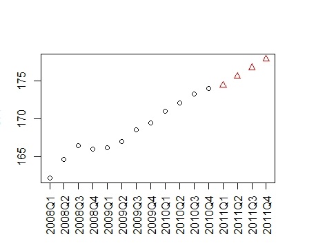
> axis(1, at=1:16, las=3,
+ labels=c(paste(year,quarter,sep="Q"), "2011Q1", "2011Q2", "2011Q3", "2011Q4"))
> iris2 <- iris
> plot(iris2[c("Sepal.Length", "Sepal.Width")], col = kmeans.result$cluster)
> iris2$Species <- NULL
> (kmeans.result <- kmeans(iris2, 3))
K-means clustering with 3 clusters of sizes 38, 50, 62
Cluster means:
Sepal.Length Sepal.Width Petal.Length Petal.Width
1 6.850000 3.073684 5.742105 2.071053
2 5.006000 3.428000 1.462000 0.246000
3 5.901613 2.748387 4.393548 1.433871
Clustering vector:
[1] 2 2 2 2 2 2 2 2 2 2 2 2 2 2 2 2 2 2 2 2 2 2 2 2 2 2 2 2
[29] 2 2 2 2 2 2 2 2 2 2 2 2 2 2 2 2 2 2 2 2 2 2 3 3 1 3 3 3
[57] 3 3 3 3 3 3 3 3 3 3 3 3 3 3 3 3 3 3 3 3 3 1 3 3 3 3 3 3
[85] 3 3 3 3 3 3 3 3 3 3 3 3 3 3 3 3 1 3 1 1 1 1 3 1 1 1 1 1
[113] 1 3 3 1 1 1 1 3 1 3 1 3 1 1 3 3 1 1 1 1 1 3 1 1 1 1 3 1
[141] 1 1 3 1 1 1 3 1 1 3
Within cluster sum of squares by cluster:
[1] 23.87947 15.15100 39.82097
(between_SS / total_SS = 88.4 %)
Available components:
[1] "cluster" "centers" "totss"
[4] "withinss" "tot.withinss" "betweenss"
[7] "size" "iter" "ifault"
> table(iris$Species, kmeans.result$cluster)
1 2 3
setosa 0 50 0
versicolor 2 0 48
virginica 36 0 14
> plot(iris2[c("Sepal.Length", "Sepal.Width")], col = kmeans.result$cluster)

+ pch = 8, cex=2)
>
> install.packages("fpc")
> library(fpc)
>
> pamk.result <- pamk(iris2)
> pamk.result$nc
[1] 2
> table(pamk.result$pamobject$clustering, iris$Species)
setosa versicolor virginica
1 50 1 0
2 0 49 50
> layout(matrix(c(1,2),1,2))
> plot(pamk.result$pamobject)

> layout(matrix(1))
> idx <- sample(1:dim(iris)[1], 40)
>
> irisSample <- iris[idx,]
> irisSample$Species <- NULL
> hc <- hclust(dist(irisSample), method="ave")
> plot(hc, hang = -1, labels=iris$Species[idx])

> rect.hclust(hc, k=3)
> groups <- cutree(hc, k=3)
> iris2 <- iris[-5]
> ds <- dbscan(iris2, eps=0.42, MinPts=5)
> table(ds$cluster, iris$Species)
setosa versicolor virginica
0 2 10 17
1 48 0 0
2 0 37 0
3 0 3 33
> plot(ds, iris2)

> plot(ds, iris2[c(1,4)])

> plotcluster(iris2, ds$cluster)


0 Comments